Monday, November 29, 2010

Median Value for Data using VBA-Macro

Thank you Abinash for coming up with a new challenge and thus something new to learn :)

I started solving it today, used references from google, applied certain code basics and was able to get the desired output.


Requirement:

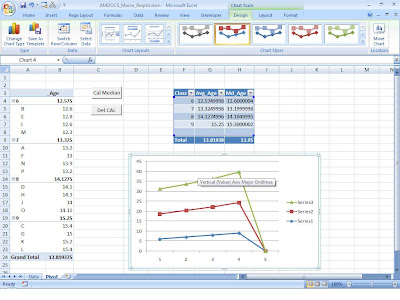
With ref to example sheet as indicated in (Snapshot 1) which stores the list of class, names of students and their ages. Create an additional field which should hold the median value of the ages grouped by class. Basically with change in the filter, when the ages are displayed as per the filtered rows, the median of the visible ages should also change.


Snapshot 1: Understanding the requirement


Snapshot-2: Knowing the solution frame-work


Snapshot-3: Observation of the result

1. click of the button Cal Median to get the desired result

2. Del CAL is used to delete the calculation and create chart.

The two buttons are added using Toolbox and are assigned macros MedianPT() and del_Chart() respectively.


Macro-code:

'---------------------------------------------------------------------------------------

'Calculation of Median (Class-wise) for a list of students

'Pivottable name -> Pivottable1

'Data in sheet "Data" name-> Table2 (It's a table and not a range)

'Result is populated in TABLE named -> Table1

'---------------------------------------------------------------------------------------

Option Explicit
Sub MedianPT()

Dim n As Integer, i As Integer, p As Integer, dt_total As Integer

Dim sr As Integer, k As Integer, j As Integer

Dim m As Single

Dim a As Variant, b As Variant, ps As Variant

Dim st As Range

Dim nn As PivotItem, pivt As PivotItem
k = 1

i = 1

p = 1

On Error GoTo 0

Application.ScreenUpdating = False
Sheets("Data").Activate

With Sheets("Data")

With .Range("Table2")

dt_total = .Rows.Count

End With
Sheets("Pivot").Activate

With ActiveSheet.PivotTables("PivotTable1")

.PivotCache.Refresh

.PivotCache.MissingItemsLimit = xlMissingItemsNone

sr = .PivotFields("Class").PivotItems.Count

ReDim ps(sr)

For n = 1 To sr

Set pivt = .PivotFields("Class").PivotItems(n)

If pivt.Visible = True Then

ps(k) = pivt.Name

k = k + 1

End If

Next n
ReDim a(dt_total, k - 1)
End With
With ActiveSheet.ListObjects("Table1") ' delete Previous Content

.ListColumns(2).DataBodyRange.ClearContents

.Range.RemoveDuplicates Columns:=2, Header:=xlYes

.ListRows(1).Range.ClearContents

.Resize .Range.Resize(sr)

.Resize .Range.Resize(k + 1)

For n = 1 To k - 1

.ListColumns(1).DataBodyRange.Cells(n) = ps(n)

Next n

End With
With ActiveSheet.PivotTables("PivotTable1")

On Error GoTo errDo

For j = 1 To k - 1

For Each nn In .PivotFields("Name").PivotItems

a(i, p) = .GetPivotData("_Age", "Class", ps(j), "Name", nn)

i = i + 1

Next nn

ReDim b(i)

For n = 1 To i - 1

b(n) = a(n, p)

Next n

m = Application.WorksheetFunction.Average(b)

Sheets("Pivot").Range("Table1[Avg_Age]").Cells(p) = m

m = Application.WorksheetFunction.Median(b)

Sheets("Pivot").Range("Table1[Md_Age]").Cells(p) = m

p = p + 1

i = 1

Next j

End With
On Error GoTo 0 'reset

m = Application.WorksheetFunction.Average(a)

ActiveSheet.ListObjects("Table1").ShowTotals = True

Range("Table1[[#Totals],[Avg_Age]]").Select

Range("Table1[[#Totals],[Avg_Age]]").Formula = "=" & m

Range("Table1[[#Totals],[Avg_Age]]").Select

m = Application.WorksheetFunction.Median(a)

Range("Table1[[#Totals],[Md_Age]]").Formula = "=" & m

End With

ActiveSheet.Shapes.AddChart.Select

ActiveChart.SetSourceData Source:=Range("Pivot!Table1")

ActiveChart.ChartType = xlLineMarkersStacked

Range("A1").Select

Exit Sub

errDo: i = i - 1
Resume Next
End Sub


Sub del_Chart()

Dim ch

ActiveSheet.ListObjects("Table1").ShowTotals = False

If ActiveSheet.ChartObjects.Count <> 0 Then

For Each ch In ActiveSheet.ChartObjects

ActiveSheet.ChartObjects.Delete

Next

Else

MsgBox "No Chart !!"

End If

With ActiveSheet.ListObjects("Table1")

.ListColumns(2).DataBodyRange.ClearContents

.Range.RemoveDuplicates Columns:=2, Header:=xlYes

.ListRows(1).Range.ClearContents

End With

End Sub


Please check the SnapShot for the data that I have:


Thursday, June 17, 2010

Sum_FromRange_AsPer_ConditionalFormatting

Anand... Thanks buddy for coming up with this Scenario... Atleast, I got a topic to post on my blog ;)

Well, There's so much that we can do with VBA but unfortunately we hardly use it in our daily work. Instead we choose the hard ways to go about it which is manual. I would urge you all to participate by coming up with Issue description wherein you need solution using VBA.
- Amit, Happy to Help! [Milind ignore the tag :)]

In this post I have used CF as an abbreviation for conditional formatting.

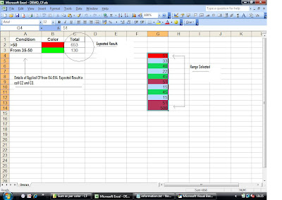
Issue Description: Sum up the values from the selected range as per the applied CF

Refer to below Snapshot


Solution:

Step 1: In the Excel file with applied CF, press Alt+f11 to open VBE and Insert MODULE

Step 2: Copy & Paste the below code of Macro Sum_As_Per_CF_Color in the MODULE

Sub Sum_As_Per_CF_Color()

Dim nbr_rows As Integer, i As Integer
Dim ftotal As Long, stotal As Long
Dim rcell As Range

ftotal = 0
stotal = 0
Set rcell = ActiveWindow.RangeSelection

nbr_rows = WorksheetFunction.Count(rcell)

Selection.Cells(1, 1).Select

For i = 1 To nbr_rows
If ActiveCell.Value > ActiveCell.FormatConditions.Item(1).Formula1 Then
ftotal = ftotal + ActiveCell.Value
Else
If (ActiveCell.Value >= ActiveCell.FormatConditions.Item(2).Formula1) And (ActiveCell.Value <= ActiveCell.FormatConditions.Item(2).Formula2) Then
stotal = stotal + ActiveCell.Value
End If
End If
ActiveCell.Offset(1, 0).Select
Next i

Cells(2, 3).Value = ftotal
Cells(3, 3).Value = stotal

End Sub


Step 3: Save the VBE Project and Press Alt+F11 to switch to EXCEL View

Step 4: Select the range with applied CF (In our eg: Select Range G4:G14)

[ Note: Applied CF details are shown from range A1 to A3 1st condition - checks if value is greater than 50 & 2nd condition- checks if value lies between 35 to 50 ]

Step 5: Go to Tools->Macro->Macros (Press Alt+F8)

Step 6: Select Sum_As_Per_CF_Color and click on Run.

Step 7: The total value as per the applied CF is displayed in cells C2 and C3 respectively.

and now we have a reason to smile... SMILE PLEASE !!

Wednesday, June 16, 2010

Sum Total as Per Cell Color

Hello All !
I Logged in after a long time.... ! Hope you all are doing good and roaring in Excel as well.
Joy... from JLT... This solution is dedicated to you. After a long time, I came across someone (Joy) who was trying to ensure that he gets all his excel issues re-solved in the short stipulated time that we got to discuss on excel. Jokes apart, Joy as I promised here is a solution that can be used for adding cell values with a particular color. Though, this will not work for cell color used by conditional formatting.

Issue Description: Sum Total the cell values as per the given cell color. In this example, as per fill color of cell C2.

Refer to the SnapShot below


Solution: Developed a Macro named Sum_As_Per_Color()

Step 1: In Your Excel File, Go To Tools->Macro->Visual Basic Editor (Shortcut: Alt+F11)
Step 2: Go To Insert->Module
Step 3: Within the inserted Module, Copy Paste the below code

Sub Sum_As_Per_Color()

Dim nbr_rows As Integer, i As Integer, val As Integer, col_nbr As Integer, row_pos As Integer
Dim total As Long

total = 0 'initialise total value to 0

'Take inputs from the User

'Nbr of rows
nbr_rows = InputBox("Enter the nbr of rows")

'Col_nbr
col_nbr = InputBox("Enter the column Index Nbr with Data")

'Row Nbr where Range Starts
row_pos = InputBox("Starting Adding from what Row Nbr?")

'Fill color of Cell C2
val = Cells(2, 3).Interior.ColorIndex

For i = 1 To nbr_rows
If Cells(row_pos, col_nbr).Interior.ColorIndex = val Then
total = total + ActiveCell.Value
End If
row_pos = row_pos + 1
ActiveCell.Offset(1, 0).Select
Next i

ActiveCell.Value = total 'Print the Final sum total in the cell below the RANGE

End Sub

Step 4: Save the File & close Visual Basic Editor
Step 5: Press Alt+F8, Run the Macro with the name Sum_As_Per_Color() and verify the result.

Note: Remember that before running the Macro, select the 1st cell from the range ie. Make it active. Also, when you run the Macro, for this example hereby is a guideline for input
1. For total nbr of rows=> 12
2. Col Index would be => 5
3. Range starts at Row Nbr=> 4

Joy & Team, Remember to ask me for lunch tommorow :).............CHEERS!!

Wednesday, May 19, 2010

Sum Every nth Data in a Range

My Struggle and at the same time great fun with Excel continues... Must say, there's something new that I learn almost everyday....

Hurray ! I got a solution to this one and this time was quick too... Bt ain't sure if this is the most efficient solution because I had to insert an additional column to get the desired result.

Scenario:
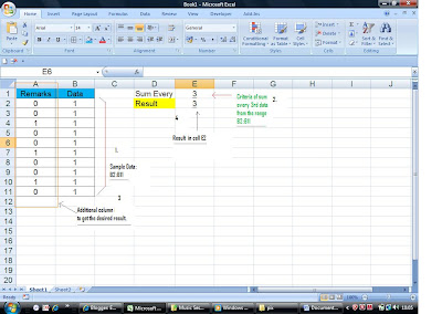
From the given range of data, user needs to sum only nth data. Say, sum every 3rd data or every 5th data, etc
Refer to the below snapshot:


From the Snapshot:
1. Sample Data
2. Cell where criteria to sum every nth data is given
3. Additional inserted column
4. Refers to cell where result is displayed

Hereby is the list of steps:
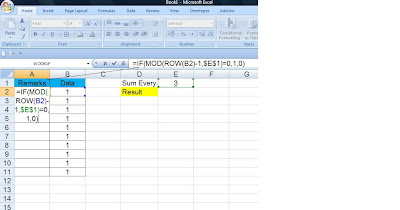
1. In the inserted additional column A, use the below formula in Cell A2:
=IF(MOD(ROW(B2)-1,$E$1)=0,1,0)


2. Copy the formula to the cell which has data in adjacent column B

Remarks: You will get 1 in every cell which matches the criteria given in cell E1.

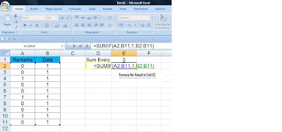
3. For Result in Cell E2, used the formula: =SUMIF(A2:B11,1,B2:B11)


4. Verify the result by changing the data in Cell E1.

Mission Accomplished !!

Sunday, May 16, 2010

Chart as per the Worksheet Name

Issues or rather room for improvement seems never ending with growing use of excel !!

Over the weekend, my client asked for a solution on excel which at the start looked very easy. But when I sat down to think about the possible solution, I was running short of ways... Thankfully, sense prevailed and I could come out with a rather easy to implement solution. It took me about 45 minutes but would definitely like to better the time taken.

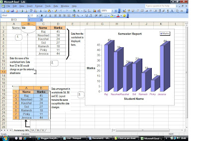
Reqmt:
To get the chart in the Summary worksheet as per the worksheet name entered in cell B2. [Example used here is with dummy data to replicate the scenario]

Challenge was to ensure that the requirement had to be solved without coding. It meant that I had to solve with just functions, cell referencing and suitable data arrangement.


Approach:
I thought of using Consolidation, 3D Referencing, data indexing, etc but to no use. Eureka !! thought of using Indirect( )

In Summary WS:
1 Worksheet name is entered in Cell B1.

2 Create Custom Type - Column with depth chart for data range from C2:D8.

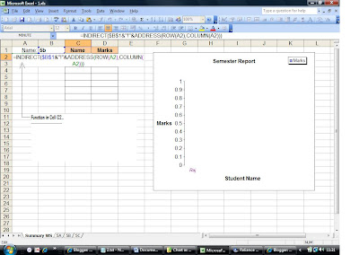
3 In the cell address c2, to get the Col A data from the worksheet as specified in cell B1, type the following function
=INDIRECT($B$1&"!"&ADDRESS(ROW(A2),COLUMN(A2)))

Drag the formula to the required number of rows from the worksheet name entered in B1


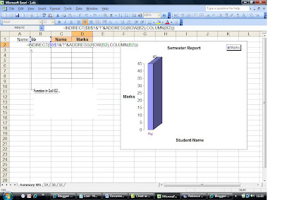
4 In the cell address d2, to get the Col B data from the worksheet as specified in cell B1, type the following function
=INDIRECT($B$1&"!"&ADDRESS(ROW(B2),COLUMN(B2)))

Drag the formula to the required number of rows from the worksheet name entered in B1


5 Verify, by giving a different worksheet name in cell B1. Data from C2: D8 should change and chart should reflect view as per the new data.

Friends, I have few consultancy work this week on EXCEL and thus, I am sure by the weekend I will have several new topics to post...

Enjoy !!

Thursday, May 13, 2010

Filter Data with Cell Fill Color

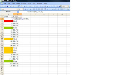
This is an interesting requirement that I came across yesterday for someone who I have given a nickname Fresher. Don't ponder for the reason, Even I don't understand why do I give such names... Anyways, let's come straight to the point.
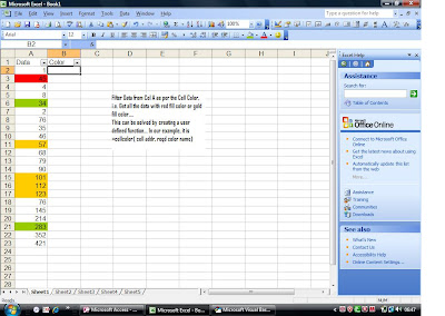
Scenario: Filter the data from Col A as per the cell fill color
Reference: Below Snapshot


Solution:
Step-wise approach:
1. ADD a new column B [Here, it's label is 'Color' at B1]
2. Create a user-defined function cellcolor() [Refer below for it's code]
3. Press Alt+F11 -> Insert -> Module -> Paste the function code here
4. Save -> Alt + Q
6. Go to cell B2, type =cellcolor(A2,true) and hit Enter
7. Drag the formula to get result for other cells i.e. applied fill color
8. Now, you can use filter drop down and select the cell color by which you want to filter data


Enjoy !! - Dedicated to Fresher...

Function Code:
Function CellColor(rCell As Range, Optional ColorName As Boolean)
Dim strColor As String, iIndexNum As Integer

Select Case rCell.Interior.ColorIndex
Case 1
strColor = "Black"
iIndexNum = 1
Case 53
strColor = "Brown"
iIndexNum = 53
Case 52
strColor = "Olive Green"
iIndexNum = 52
Case 51
strColor = "Dark Green"
iIndexNum = 51
Case 49
strColor = "Dark Teal"
iIndexNum = 49
Case 11
strColor = "Dark Blue"
iIndexNum = 11
Case 55
strColor = "Indigo"
iIndexNum = 55
Case 56
strColor = "Gray-80%"
iIndexNum = 56
Case 9
strColor = "Dark Red"
iIndexNum = 9
Case 46
strColor = "Orange"
iIndexNum = 46
Case 12
strColor = "Dark Yellow"
iIndexNum = 12
Case 10
strColor = "Green"
iIndexNum = 10
Case 14
strColor = "Teal"
iIndexNum = 14
Case 5
strColor = "Blue"
iIndexNum = 5
Case 47
strColor = "Blue-Gray"
iIndexNum = 47
Case 16
strColor = "Gray-50%"
iIndexNum = 16
Case 3
strColor = "Red"
iIndexNum = 3
Case 45
strColor = "Light Orange"
iIndexNum = 45
Case 43
strColor = "Lime"
iIndexNum = 43
Case 50
strColor = "Sea Green"
iIndexNum = 50
Case 42
strColor = "Aqua"
iIndexNum = 42
Case 41
strColor = "Light Blue"
iIndexNum = 41
Case 13
strColor = "Violet"
iIndexNum = 13
Case 48
strColor = "Gray-40%"
iIndexNum = 48
Case 7
strColor = "Pink"
iIndexNum = 7
Case 44
strColor = "Gold"
iIndexNum = 44
Case 6
strColor = "Yellow"
iIndexNum = 6
Case 4
strColor = "Bright Green"
iIndexNum = 4
Case 8
strColor = "Turqoise"
iIndexNum = 8
Case 33
strColor = "Sky Blue"
iIndexNum = 33
Case 54
strColor = "Plum"
iIndexNum = 54
Case 15
strColor = "Gray-25%"
iIndexNum = 15
Case 38
strColor = "Rose"
iIndexNum = 38
Case 40
strColor = "Tan"
iIndexNum = 40
Case 36
strColor = "Light Yellow"
iIndexNum = 36
Case 35
strColor = "Light Green"
iIndexNum = 35
Case 34
strColor = "Light Turqoise"
iIndexNum = 34
Case 37
strColor = "Pale Blue"
iIndexNum = 37
Case 39
strColor = "Lavendar"
iIndexNum = 39
Case 2
strColor = "White"
iIndexNum = 2
Case Else
strColor = "No Fill "
End Select

If ColorName = True Or strColor = "Custom color or no fill" Then
CellColor = strColor
Else
CellColor = iIndexNum
End If

End Function

Tuesday, May 11, 2010

Introduction


The reason I felt the need of creating a blog is to share my knowledge with you on Microsoft Application EXCEL. Being in the corporate world for over 6 years has been great and much to my delight. I always got to learn something new. Also, got certified with Microsoft on EXCEL 2007 (MCAS) which was definitely fun. 3 years back, I knew not much about Excel except for the very basics that it's used to store data in tabular format, etc. I used to wonder if there were ways to store data in a systematic and useful manner on Excel. But, one of the requirements of my client changed my ways of thinking. One of the highlight of my career is that in short span of 6 years in IT, I got a chance to interact with over 60 Companies, 10K Professionals. Thanks to my approach of consulting.

To begin with, I would post blog on topics from EXCEL to cover the Basic, Intermediate and Advance concepts. Going forward, would stress upon Data Handling tips and tricks on Excel.

This blog is dedicated to all of you who wants to learn more about Excel and unravel the ways to efficiently use its features.

Incase of any suggestions, please feel free to post.

-Thank you (धन्यवाद)