Chart as per the Worksheet Name

Issues or rather room for improvement seems never ending with growing use of excel !!

Over the weekend, my client asked for a solution on excel which at the start looked very easy. But when I sat down to think about the possible solution, I was running short of ways... Thankfully, sense prevailed and I could come out with a rather easy to implement solution. It took me about 45 minutes but would definitely like to better the time taken.

Reqmt:
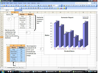
To get the chart in the Summary worksheet as per the worksheet name entered in cell B2. [Example used here is with dummy data to replicate the scenario]

Challenge was to ensure that the requirement had to be solved without coding. It meant that I had to solve with just functions, cell referencing and suitable data arrangement.



Approach:
I thought of using Consolidation, 3D Referencing, data indexing, etc but to no use. Eureka !! thought of using Indirect( )

In Summary WS:
1 Worksheet name is entered in Cell B1.

2 Create Custom Type - Column with depth chart for data range from C2:D8.

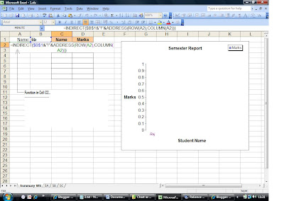
3 In the cell address c2, to get the Col A data from the worksheet as specified in cell B1, type the following function
=INDIRECT($B$1&"!"&ADDRESS(ROW(A2),COLUMN(A2)))

Drag the formula to the required number of rows from the worksheet name entered in B1




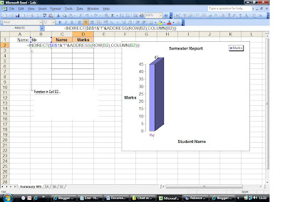
4 In the cell address d2, to get the Col B data from the worksheet as specified in cell B1, type the following function
=INDIRECT($B$1&"!"&ADDRESS(ROW(B2),COLUMN(B2)))

Drag the formula to the required number of rows from the worksheet name entered in B1



5 Verify, by giving a different worksheet name in cell B1. Data from C2: D8 should change and chart should reflect view as per the new data.

Friends, I have few consultancy work this week on EXCEL and thus, I am sure by the weekend I will have several new topics to post...

Enjoy !!